Introduction

Employee wellbeing is a concern in occupational psychology. Negative antecedents such as toxic work environments, poor organisational climate, bullying, amount and type of working hours among many others (Colligan & Higgins, 2006), increase employee stress. The addition of the Covid-19 pandemic brings new stressors, such as changing working practices by working from home or being on furlough, which have helped contribute to what has become known as “The Great Resignation” (TGR).

It would seem that the pandemic has allowed some people to re-evaluate their lives and working practices, thereby, looking after their own wellbeing by doing what is best for them. Though these might be troubling times as far as some employees or organisations are concerned, some recruitment writers see suitable benefits for how TGR can potentially benefit your career and consequently increase wellbeing.

However, this is not an essay or report on wellbeing in the workplace. The subject is far too deep and complicated to go into here in any great detail, but the introduction sets the scene.

The idea here is to investigate the relationships between wellbeing and working hours using the lessr package (Gerbing, 2021) which I have recently found to be very useful.

The Data

The wellbeing data are included in the UsingR package and originally found here, where you can see interactive correlations with wellbeing and variables of your choice. There are also links to the data origin at The National Accounts of Well-being and category data from Gapminder, where you can also download other data from the Gapminder database in CSV or XLSX formats.

The wellbeing data consists of \(22\) observations (European countries):

Austria, Belgium, Bulgaria, Cyprus, Denmark, Estonia, Finland, France, Germany, Hungary, Ireland, Netherlands, Norway, Poland, Portugal, Slovakia, Slovenia, Spain, Sweden, Switzerland, Ukraine, United Kingdom

and \(11\) additional variables:

Well.being, GDP, Equality, Food.consumption, Alcohol.consumption, Energy.consumption, Family, Working.hours, Work.income, Health.spending, Military.spending

The data require minimal cleaning, so in this case only the necessary columns are selected with d[] function; and the Well.being column sorted with the Sort() function in lessR. For the purposes of using lessR, the UsingR::wellbeing data frame was saved as an .xlsx file with Write() and re-imported with Read() into the variable d (you might not have to do this - I could not get the original data to be manipulated with lessR functions).

The Analysis

Table 1 shows the top five European countries with the highest wellbeing (Denmark: 5.93), and the bottom five with the lowest wellbeing (Ukraine: 4.39). There’s not much difference between the highest and lowest positions (1.54).

Highest Wellbeing

Lowest Wellbeing

Table 1.
European Countries with Highest & Lowest Wellbeing

Country	Well.being	Working.hours
Denmark	5.93	30.27
Norway	5.69	27.08
Switzerland	5.66	31.87
Ireland	5.44	31.54
Sweden	5.44	30.30

Country	Well.being	Working.hours
Estonia	4.80	NA
Hungary	4.74	38.25
Bulgaria	4.59	NA
Slovakia	4.57	33.63
Ukraine	4.39	NA

Note:

Working.hours are the average working hours per week per person

Not all functions from lessr are necessary for this project. So aside from the “tidying” functions used above, the additional functions of interest are Regression() and regPlot().

The Regression() function is really useful. As the name lessR suggests, less \(R\) and more output. We want to explore the relationship between wellbeing (Intercept) and the average working hours per week per person (predictor). The output for Regression() includes everything you need (and more), all of which can be presented separately if assigned to its own variable, such as:

The regression estimate:

##                Estimate    Std Err  t-value  p-value   Lower 95%   Upper 95%
##   (Intercept)      7.08       0.83    8.571    0.000        5.32        8.84
## Working.hours     -0.06       0.03   -2.279    0.038       -0.11       -0.00

The Anova:

## -- Analysis of Variance
## 
##                 df    Sum Sq   Mean Sq   F-value   p-value
## Model            1      0.58      0.58      5.20     0.038
## Residuals       15      1.68      0.11
## Well.being      16      2.27      0.14

The adjusted R-squared value is \((R_{adj}^2 = 0.2077)\).

The statistical information is reported as follows:

A simple linear regression was carried out to test if Working Hours significantly predicted Wellbeing. The results of the regression indicated that the model explained 20.77% of the variance and that the model was significant, \(F\)(1, 15) \(=\) 5.2, \(p=\) 0.038. It was found that Working Hours significantly predicted Wellbeing (\(B_1=\) -0.06, \(p=\) 0.038).
The final predictive model is: proportion of Wellbeing \(=\) 7.08 + (-0.06 \(\times\) Working Hours)

Plots

Three plots for visualising the regression and the assumptions are also produced (automatically in the Regression() function, or separately using regPlot()), as here:

Figure 1.
Scatterplot showing regression line, prediction and confidence intervals:

Figure 2.
Bar/density plot for distribution of residuals

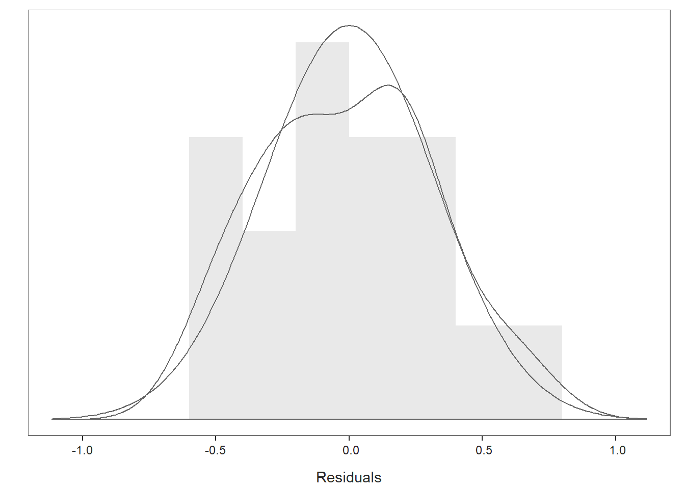
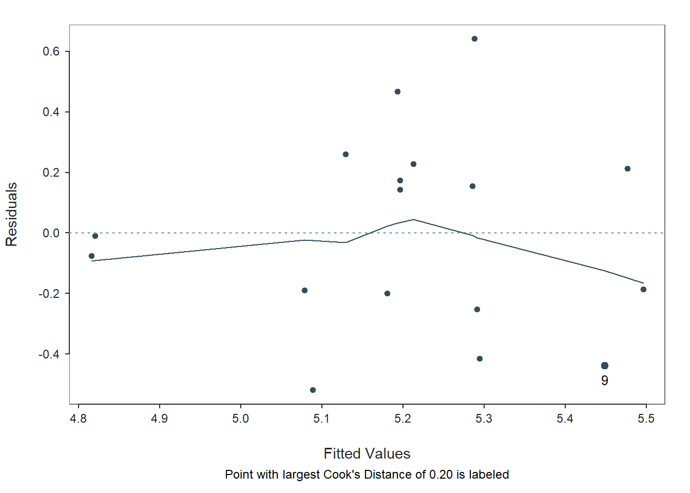
Figure 3.
Scatterplot for residuals vs. fitted values

Additional Output

Additional analyses of interest in the Regression() output are the correlation matrix, which shows a negative moderate relationship between wellbeing and working hours \((r= -0.51)\):

RELATIONS AMONG THE VARIABLES:

##                 Well.being Working.hours
##      Well.being       1.00         -0.51
##   Working.hours      -0.51          1.00

RESIDUALS AND INFLUENCE (Top five showing here)

##  [1] "-- Data, Fitted, Residual, Studentized Residual, Dffits, Cook's Distance"
##  [2] "   [sorted by Cook's Distance]"                                          
##  [3] "   [n_res_rows = 17, out of 17 ]"                                        
##  [4] "--------------------------------------------------------------"          
##  [5] "     Working.hours Well.being fitted resid rstdnt dffits cooks"          
##  [6] "   9         27.55       5.01   5.45 -0.44  -1.49  -0.65  0.20"          
##  [7] "   5         30.27       5.93   5.29  0.64   2.24   0.62  0.15"          
##  [8] "  16         33.63       4.57   5.09 -0.52  -1.72  -0.51  0.12"          
##  [9] "  20         31.87       5.66   5.19  0.47   1.50   0.37  0.06"          
## [10] "   8         30.16       4.88   5.29 -0.41  -1.32  -0.37  0.06"

PREDICTION ERROR

– Data, Predicted, Standard Error of Prediction, 95% Prediction Intervals [sorted by lower bound of prediction interval] ———————————————-(Top 5 again)

## [1] "     Working.hours Well.being pred s_pred pi.lwr pi.upr width"
## [2] "  10         38.25       4.74 4.82   0.38   4.00   5.64  1.64"
## [3] "  14         38.17       4.81 4.82   0.38   4.00   5.64  1.64"
## [4] "  15         33.81       4.89 5.08   0.35   4.33   5.82  1.49"
## [5] "  16         33.63       4.57 5.09   0.35   4.35   5.83  1.49"
## [6] "   7         32.95       5.39 5.13   0.35   4.39   5.87  1.48"

Another excellent feature of the Regression() function is the Rmd = "filename" parameter which automatically produces an explanatory and exploratory .Rmd document of the regression analysis that can be edited; and an additional .html document, which for this analysis you can read here.

Further Query

Clearly, working more hours in a week reduces wellbeing. We have already seen that the Wellbeing Mean for this data set is \(5.1\). This could be considered as peak wellbeing, so what are the average working hours per week per person needed to maintain that level of wellbeing?

The prediction output suggests a level of wellbeing at \(5.13\) \((95\%\space CI[4.39, 5.87])\) for \(32.95\) (round to \(33\)) average hours worked at item \(7\):

## [1] "     Working.hours Well.being pred s_pred pi.lwr pi.upr width"
## [2] "   7         32.95       5.39 5.13   0.35   4.39   5.87  1.48"

This prediction can be confirmed with the regression calculation identified above:

Wellbeing = 7.08 + (-0.06 \(\times\) Working Hours) \(\space\therefore\space\) 7.08 + (-0.06 \(\times\) 33) \(=\) 5.13

If the preferred working hours to maintain wellbeing at \(5.13\) is \(33\), then the question is: would it be more beneficial to work a shorter week with longer hours per day, or a longer week with fewer hours per day? See Table 2 (Calculations converted to time with lubridate (Spinu et al., 2023)).

**Table 2.**
*Speculative Working Week*
Days per Week	Hours per Day
4	8H 15M 0S
5	6H 36M 0S

Of course there are other options, for example, a three day week at \(11\) hours per day, or a six day week at \(5\) hours \(30\) minutes per day, not intending to dismiss those workers who would do more (or less).

This theory does not account for the four countries that work fewer than \(33\) hours per week per person and have a lower than average wellbeing: Belgium, France, Germany and the United Kingdom (See the lower-left quadrant of Figure 1; and Table 3).

**Table 3.**
*European Countries with Wellbeing < 5.13 and Working Hours < 33*
Country	Well.being	Well.being.diff	Working.hours	Working.hours.diff
Belgium	5.04	-0.09	30.21	-2.79
France	4.88	-0.25	30.16	-2.84
Germany	5.01	-0.12	27.55	-5.45
United Kingdom	4.98	-0.15	32.09	-0.91

In this group, France has the largest difference in wellbeing \((-0.25)\), a \(1/4\) of a point less than average wellbeing. However, all of the wellbeing differences are very small; and the wellbeing scores for each country are within the bounds of the \(95\%\space CI[4.39, 5.87]\) of the wellbeing/working hours prediction. The country with the greatest working hours difference is Germany at \(-5.45\), which is \(5\) hours \(27\) minutes fewer than average. Further research is required to determine the whys and wherefores, which is beyond the scope of this report.

Conclusion

A very brief introduction to employee wellbeing preceded the purpose of using various functions from the lessR package to explore the relationship between Well.being and Working.hours in \(22\) European countries using the UsingR::wellbeing data set. The lessR functions used were Write(), Read(), d[], Sort(), Regression() and regPlot(). The key Regression() outputs, estimate, ANOVA and adjusted R-squared were presented separately to weave into the text, along with three plots to verify regression assumptions. Additional output for correlation, residuals and influence and prediction error followed. Further query suggested a predicted number of average working hours to maintain average wellbeing, with speculative thought on how a working week could be arranged. Finally, the four countries showing less than wellbeing average and fewer than average working hours were addressed. In general, lessR was found to be an excellent \(R\) package to manipulate data with minimal use of \(R\) for maximum output.

References

Colligan, T. W., & Higgins, E. M. (2006). Workplace stress: Etiology and consequences. Journal of Workplace Behavioral Health, 21(2, 2), 89–97. https://doi.org/10.1300/J490v21n02_07

Gerbing, D. W. (2021). Enhancement of the command-line environment for use in the introductory statistics course and beyond. Journal of Statistics and Data Science Education, 29(3), 251–256. https://doi.org/10.1080/26939169.2021.1999871

Spinu, V., Grolemund, G., & Wickham, H. (2023). Lubridate: Make dealing with dates a little easier. https://lubridate.tidyverse.org

Using the `lessR` package to investigate wellbeing data

Stuart Leeds

01/12/2021

Introduction

The Data

The Analysis

Plots

Additional Output

Further Query

Conclusion

References

Using the lessR package to investigate wellbeing data

Stuart Leeds

01/12/2021

Introduction

The Data

The Analysis

Plots

Additional Output

Further Query

Conclusion

References

Using the `lessR` package to investigate wellbeing data